Word clouds, train/test splitting, four classification models, SMOTE oversampling,
and a full performance comparison before and after SMOTE.
3a
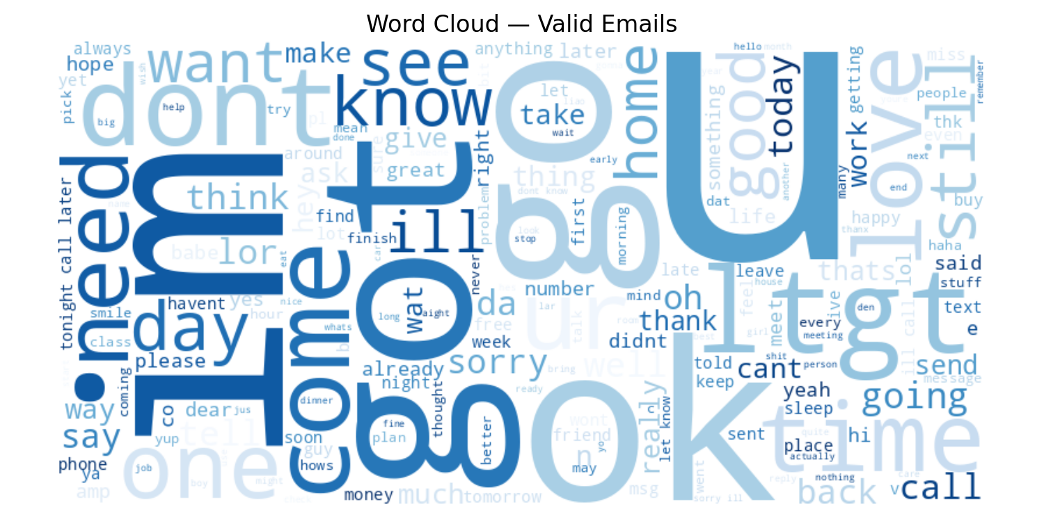
Word Clouds
After preprocessing, the most frequent words in each class are visualized.
The size of each word is proportional to its frequency in that class's corpus.
Valid emails — dominated by conversational words:
call, good, know, time, come, will. Natural, personal language.
Spam emails — dominated by urgency and reward words:
free, call, claim, text, prize, win. Manipulative, transactional language.
3b
Data Splitting
The dataset is split into a training set (80%) used to
fit the models, and a test set (20%) held out for
unbiased evaluation. Stratification ensures the spam/valid ratio is preserved in both splits.
from sklearn.model_selection importtrain_test_split
X_train, X_test, y_train, y_test = train_test_split(
X_all, y_all,
test_size=0.2, # 20 % held out for evaluation
random_state=42, # reproducibility
stratify=y_all, # preserves class ratio in both splits
)
Training Set
4,457
80% · used to fit models
Test Set
1,115
20% · held out for evaluation
3c — Round 1
Models Before SMOTE
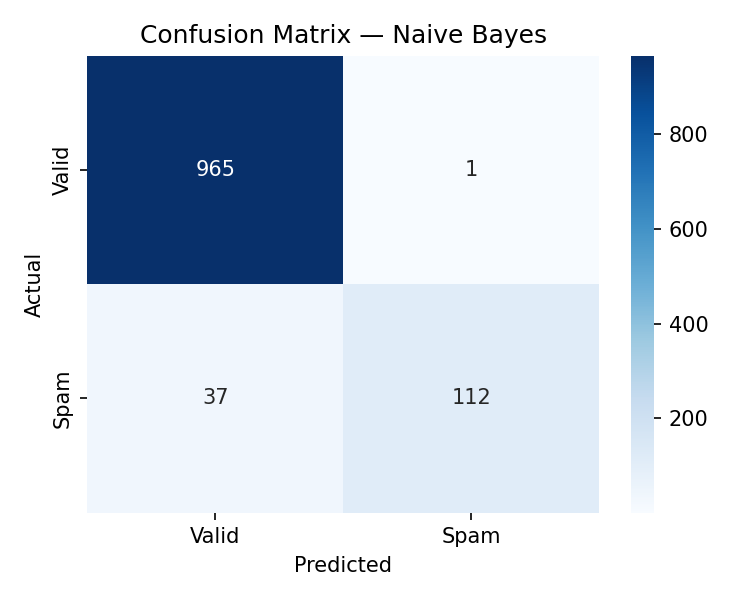
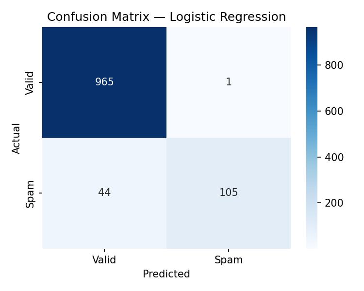
Four classifiers are trained on the original imbalanced training set.
Each model is evaluated on the held-out test set with a confusion matrix.
Instance-based
K-Nearest Neighbors
F1 87.2%
Classifies by majority vote of the 5 nearest training examples, measured by cosine similarity between TF-IDF vectors.
The training set contains only 13.4% spam messages. Models trained on imbalanced data
tend to favor the majority class (valid), resulting in poor spam recall.
SMOTE (Synthetic Minority Over-sampling Technique)
resolves this by generating synthetic spam samples in the feature space.
Before SMOTE
Valid3,565
Spam892
Heavily imbalanced — 20% spam
After SMOTE
Valid3,566
Spam (+ synthetic)3,566
Balanced — 50/50 split
from imblearn.over_sampling importSMOTE
smote = SMOTE(random_state=42)
X_train_sm, y_train_sm = smote.fit_resample(X_train, y_train)
# Result: training set grows from 4,457 → 7,132 samples# Both classes now have exactly 3,566 examples
3e — Round 2
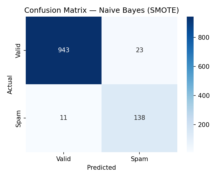
Models After SMOTE
The same four models are retrained on the SMOTE-balanced training set
and evaluated on the same original test set.
All metrics are measured on the held-out 20% test set. F1 scores reflect spam-class performance.
Key finding: SMOTE improved spam recall for 3 of 4 models.
Logistic Regression improved the most
(+9.2% F1).
KNN was the only model to decline slightly
(-3.3% F1).
Random Forest achieved the highest absolute F1 after SMOTE at
93.6%.